Dual-Slope Energy Metering Circuits: How Interference Disrupts Positive Integration, Negative Integration and Pulse Output

Electromagnetic interference can affect an integrating measurement circuit in three main ways: it changes the integrated input, alters the reference-driven return ramp, or disrupts conversion timing and pulse reception. The first two can change a conversion result without stopping the circuit. Pulse interruptions can follow when conversion cannot finish, the controller resets, or the output path stops transferring valid signals.

A blinking—or stationary—pulse indicator cannot identify which mechanism is responsible. The useful explanation connects three things: where interference enters, how the integration waveform changes, and how that change reaches the measurement result or pulse output.

Model and scope: This article uses a typical dual-slope model. “Positive integration” means input integration; “negative integration” means de-integration with an opposing reference. These names do not require the output to become positive and then negative, imply two independent channels, or describe import/export energy registers. To explain the metering consequences, assume that a front end has already produced a low-bandwidth signal proportional to active power. Conversion results then feed time-weighted energy accumulation and pulse generation; this assumes the measured power represents the interval assigned to it, including any gaps between conversions. This is an explanatory model, not a universal energy-meter architecture; sigma-delta ADCs, digital multiplication and direct voltage-to-frequency conversion require analysis of their actual signal paths. Waveform checks are for qualified engineers using appropriately rated isolated measurement arrangements: a metering board may be referenced to mains voltage, so an ordinary earth-referenced oscilloscope ground must not be connected to a live-referenced node.

1. Normal Operation: What Happens During a Dual-Slope Conversion?

Separate the analog conversion from the energy-pulse function:

Power-proportional signal
        ↓
Input/reference switching → Integrator → Comparator → Timing and conversion result
        ↑                                              │
        └──────────────── Phase control ────────────────┘

Conversion result → Time-weighted energy accumulation
                  → One pulse's energy increment reached → Metering pulse

These are functional relationships, not wiring instructions. The comparator’s conversion-complete transition is not the metering pulse generated downstream.

Positive Integration: Convert the Input Into a Voltage Excursion

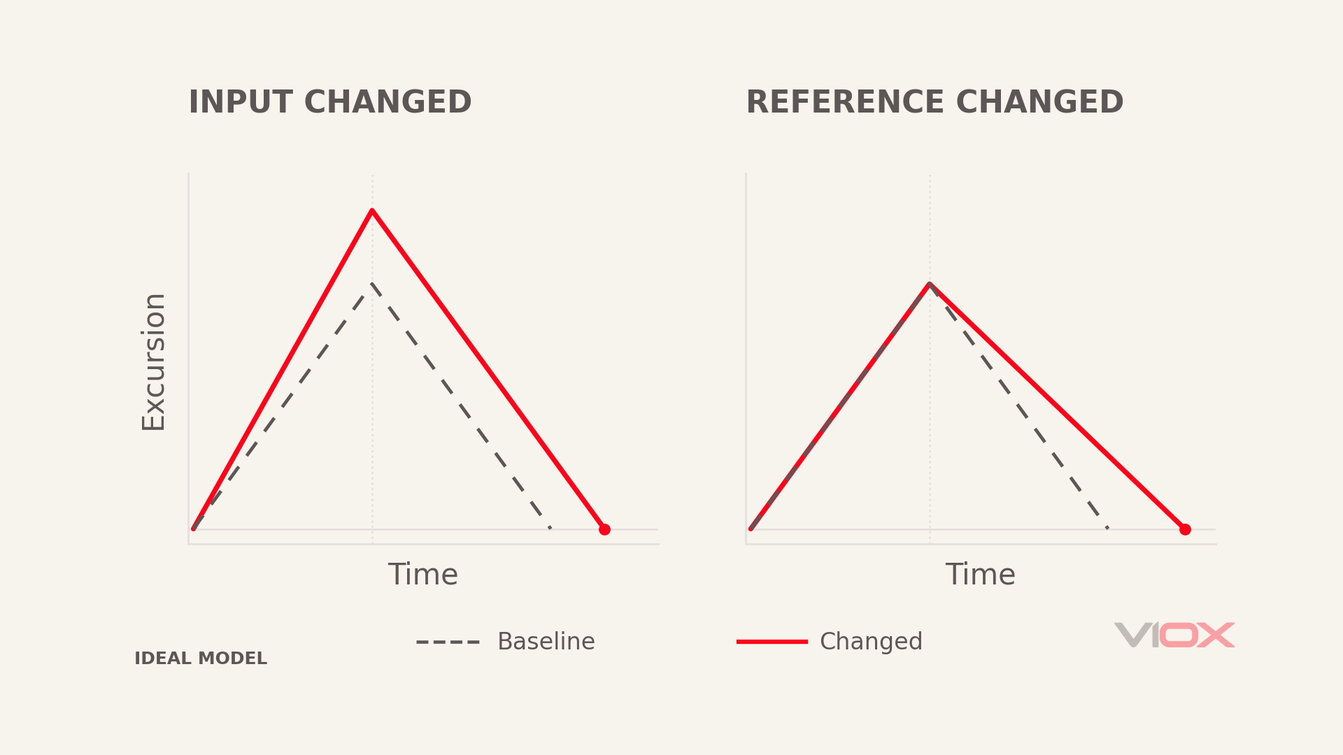
Input integration lasts for a fixed interval, T₁. For a constant input, the magnitude of the ideal integrator’s output excursion is:

|ΔV₁| = |Vin| × T₁ / (Rint × Cint)

A larger input produces a steeper ramp. A longer integration interval produces a larger excursion. For a changing input, the final excursion depends on the input’s area over the integration window, not on a single instantaneous peak.

Here, ΔV is a voltage change. The corresponding charge change is ΔQ = Cint × ΔV; the two quantities are not interchangeable.

Negative Integration: Return to the Starting Threshold at a Known Slope

After input integration, the circuit switches to a reference that drives the output back toward its starting threshold. The ideal return-slope magnitude is:

|S₂| = |Vref| / (Rint × Cint)

If both phases use the same Rint and Cint and return to the same threshold:

|Vin| × T₁ = |Vref| × T₂

Therefore:

T₂ = T₁ × |Vin| / |Vref|

A normal conversion has two ramps: one moves away from the starting point; the other returns toward it. The comparator detects the return threshold, allowing the controller to stop timing T₂.

For an illustrative input of 0.5 V, reference magnitude of 1 V and T₁ of 20 ms, the ideal T₂ is 10 ms. These are calculation inputs, not specifications for a particular meter.

Dual-slope conversion allows the ideal values of the shared RC components to cancel from the ratio. Offset, leakage, threshold error and overload recovery still matter. Practical implementations may include auto-zero and residual-clearance phases. See Analog Devices’ explanation of integrating ADC architectures.

2. Where Does Interference Enter—and What Does It Change?

The same external disturbance can produce different results depending on the node it reaches.

Coupling location	Circuit quantity affected	Immediate symptom
Sampling and integrator input	Input voltage, current or integrated area	Ramp-slope change or endpoint shift
Supply, reference and reference ground	Amplifier headroom, return slope or comparison threshold	Clipping, changed return time or endpoint jitter
Switch control, clock and reset	Phase duration, switching time or valid timer count	Conversion jumps, timeouts or restarts
Pulse driver and receiver interface	Logic levels, pulse width, edges or receiver reference	False pulses, missed counts or missing external pulses

A common-mode disturbance moving both input terminals together is not automatically a differential measurement error. However, finite common-mode rejection, mismatched input-filter impedances or an exceeded common-mode range can allow it to affect the result.

Also distinguish a temporary error during interference, recovery after the event, and lasting hardware damage. A brief pause in the output does not establish permanent component failure.

Clock errors also need context. If the fixed integration interval and return count use the same stable clock, a common clock-frequency scale factor cancels from their ratio. A clock disturbance between phases, a lost edge or a reset can still corrupt a conversion. Separately, energy accumulation depends on elapsed time: conversion-ratio cancellation does not guarantee an accurate energy time base.

3. Positive-Integration Faults: Why Does the Ramp Change, Clip or Stop?

Input Interference Is Integrated Along With the Signal

Suppose the actual input consists of the wanted signal Vin(t) plus a disturbance vn(t). For an ideal inverting integrator, the disturbance contributes an additional output excursion:

δV₁ = −[1 / (Rint × Cint)] × ∫ vn(t) dt, integrated from 0 to T₁

The immediate implication is useful: the disturbance’s net area within the integration window determines this contribution to conversion error.

If its positive and negative areas cancel, the endpoint error can be small. If the window covers only part of a cycle, or the disturbance contains an offset, the endpoint shifts. A fixed integration interval can reject certain periodic disturbances through averaging; it does not automatically remove every high-frequency signal.

There is another path. High-frequency interference can be rectified by nonlinear junctions in the front end, creating a low-frequency or DC error. The integrator then receives an already-distorted signal. Extending the integration interval alone may not remove that error. Analog Devices tutorial MT-096 explains RF rectification in precision amplifiers.

Evidence to look for: the input phase starts and finishes normally, but its endpoint and subsequent return time change with the input disturbance. First establish whether the input area changed or the integrator itself stopped behaving linearly.

Insufficient Headroom Clips the Ramp

The linear integration relationship applies only while the amplifier remains within its specified operating conditions.

An excessive input, or a supply disturbance that reduces available output swing, can drive the ramp to the amplifier’s output limit. The waveform develops a plateau. Input may still be present, but the output no longer follows the expected slope, so the conversion loses information about the input area.

That differs from a flat ramp caused by a genuinely zero input. Compare the input, supply and integrator output together:

• Input present, output near its swing limit: investigate headroom or overload.
• Input not actually connected, output holding its previous value: inspect the switching state and input path.
• Abnormal behavior continues briefly after normal conditions return: evaluate overload recovery before concluding that the amplifier is damaged.

Common-mode overrange, output saturation and CMOS latch-up are different conditions. A latch-up diagnosis requires evidence such as device-specific behavior, abnormal current and recovery characteristics—not just a flat waveform.

Switching and Leakage Alter the Integrating Current

Analog-switch transitions can inject charge. If a net charge ΔQ reaches the integrating capacitor, the resulting voltage step is approximately:

ΔVstep ≈ ΔQ / Cint

This often appears as a step at the switching instant rather than a uniform change in slope. Charge distribution depends on the switch and surrounding circuit; the entire datasheet charge-injection value should not automatically be assigned to Cint. See Analog Devices’ analog-switch tutorial MT-088.

A sustained additional leakage current behaves more like an extra input. Its slope-error magnitude is approximately |Ileak| / Cint. When the wanted input current is small, the same leakage produces a larger relative error.

Charge injection and leakage are existing circuit nonidealities. Establish whether external interference worsens them by comparing waveforms, operating conditions and device behavior before, during and after the event.

4. Negative-Integration Faults: Why Does the Return to Threshold Go Wrong?

Reference Variation Changes the Return Speed

With the input-integration endpoint unchanged, a smaller reference magnitude produces a shallower return ramp and a longer T₂. A larger reference magnitude does the opposite.

For a small reference change that remains approximately constant during de-integration, the inverse relationship gives:

δT₂ / T₂ ≈ −δVref / Vref

Here, Vref denotes the reference magnitude. If downstream processing still uses the nominal reference value, a longer T₂ is interpreted as a larger input. The first consequence is a gain error, not necessarily a stopped pulse output.

If the reference varies throughout de-integration, the return slope varies with time. Evaluate the reference’s integral over that phase rather than relying on one instantaneous voltage reading.

The Reference Is Not Applied Correctly

The controller may command de-integration without establishing the intended reference current. The output can then hold, drift slowly, or respond mainly to leakage and bias. Incorrect reference polarity can drive it farther from the endpoint.

The decisive observation is: after the switching command, does the integrating node actually receive current in the required direction?

This is more informative than attributing a high output to a collapsed negative supply. De-integration needs an opposing current; whether the circuit requires a separate negative supply depends on its implementation.

Threshold Noise Corrupts the End-of-Conversion Event

A comparator responds to the difference between its two inputs. Near the endpoint, noise on the ramp or comparison reference can change the sign of that difference repeatedly. The resulting transition may be early, late or repeated. Texas Instruments’ comparator-with-hysteresis guidance describes multiple transitions caused by noise near a threshold.

For a small effective threshold error δV and an approximately constant endpoint slope, the timing-error magnitude is:

|δt| ≈ |δV| / |S₂|

The same voltage disturbance therefore creates a larger timing error when the return ramp is slower.

What happens next depends on the control logic. Capturing an early edge shortens the measured interval. Missing the valid edge can delay completion or trigger a timeout. Indefinite waiting depends on the implementation’s timeout and recovery behavior; it is not an inevitable “comparator lockup.”

Observe the integrator output, comparator output and conversion-complete state on the same time base. That distinguishes an analog return fault from a missed digital event.

Capacitor Memory and Residue Change the Next Starting Point

Dielectric absorption makes capacitor behavior depend on previous charge and discharge history. Incomplete residual clearing can also leave the next conversion starting from a different level. These errors may become more noticeable after an input-amplitude or polarity change.

The Microchip TC500-family documentation describes a residual-clearing phase and requires low dielectric absorption in the integrating capacitor. Evaluate the error budget, leakage and history-dependent behavior. A dielectric label alone does not establish that an integrator will enter permanent saturation after a few cycles.

5. How Do Integration Faults Become Metering-Pulse Errors?

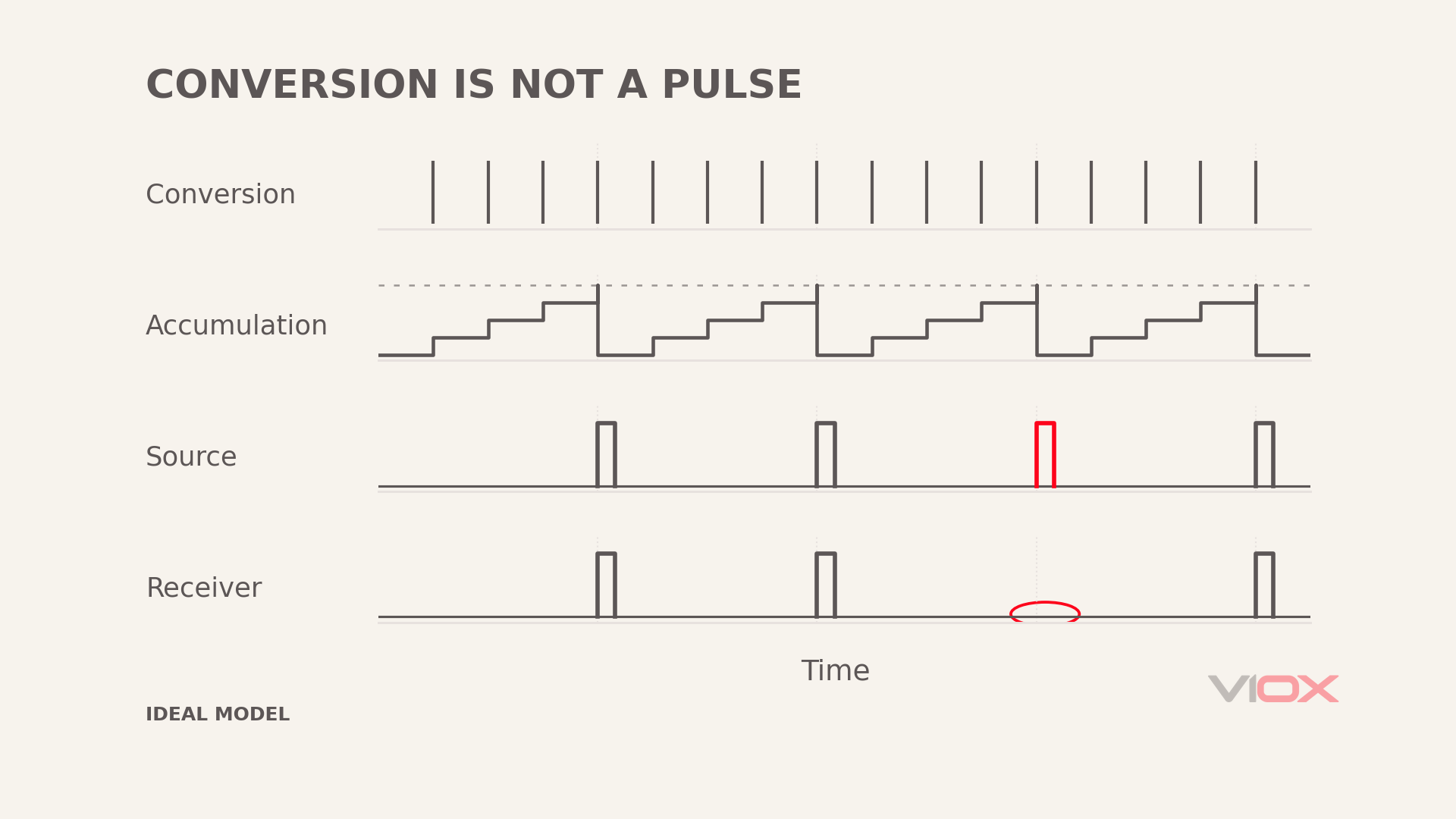
In the model used here, each valid conversion provides a power estimate, P̂. Downstream processing accumulates energy using the associated time interval: ΔE = P̂ × Δt, with power in kW and time in hours for energy in kWh. Simply counting completed conversions would not perform this function, especially when return times vary. Once the accumulator reaches one pulse’s energy increment, it emits a pulse and retains the remainder.

A calibration-frequency (CF) pin and an isolated meter pulse terminal may use different scaling or operating rules. Use the pulse constant and enable/no-load conditions for the particular output being observed.

For a pulse constant K in impulses/kWh and steady nonnegative active power P in kW for the selected energy direction, the ideal average pulse frequency is:

f = K × P / 3600 Hz

This separates four possible outcomes.

Pulse Frequency Is Too High or Too Low

An input-area error, reference change or endpoint-timing error can alter the power estimate. A sustained bias then changes the average pulse frequency.

Downstream averaging may reduce random jitter, whereas a persistent signed bias can continue accumulating. A change in one pulse interval alone does not establish the long-term energy error. At low power, the expected interval can itself be long: for an illustrative K of 1,000 impulses/kWh and P of 0.01 kW, the ideal average interval is 360 seconds, provided the output is enabled and above its no-load threshold.

Pulse Output Is Interrupted Intermittently

A conversion timeout, supply reset or interrupted phase sequence can delay new data entering the energy accumulator. Whether pulses stop immediately depends on how the system handles invalid data: discarding it, holding the previous value or suspending measurement.

There is consequently no fixed one-to-one relationship between an abnormal conversion and a lost metering pulse.

Pulse Output Stops Persistently

Conversion may never complete, the controller may remain in reset, pulse generation may be disabled, or the output interface may fail.

Actual metering ICs can also suppress pulses intentionally under defined conditions. For example, the ADE7755 datasheet describes pulse suppression during undervoltage reset and no-load operation. This is evidence of output behavior, not an example of a dual-slope converter.

The Receiver Overcounts or Undercounts

A disturbance at the output interface can create extra threshold crossings and false counts. It can also alter the signal level or pulse width so that a valid pulse no longer meets the receiver’s requirements. Excessive input filtering can reject legitimate narrow pulses as well.

Compare the source and receiver. A correct source waveform with incorrect received counts redirects the investigation to the interface. VIOX’s pulse-counter guide provides related background on counting and input conditions.

6. Connect the Symptom, Mechanism and Evidence

Observed symptom	Candidate disturbance path	Evidence needed
Input-integration endpoint shifts, but the ramp remains continuous	Input disturbance, offset or extra leakage	Corresponding changes in input area, endpoint and return time
Input-integration ramp clips	Input overload or insufficient output headroom	Actual input, supply and output-swing limits
A step appears at switching	Charge injection or control-signal coupling	Timing of the step relative to the switching edge
De-integration slows but completes	Changed reference or return current	Agreement between reference, ramp slope and T₂ changes
No return trend during de-integration	Reference path or switch-state fault	Commanded state compared with the actual node response
Ramp crosses the endpoint, but conversion times out	Comparator, capture or control-state problem	Sequence of analog crossing, digital edge and completion state
Pulse interruption coincides with reset	Supply or reset path	Time correlation between the supply event, reset and missing pulses
Source pulses are present, but the receiver misses counts	Driver, isolation, cable or input configuration	Levels, widths, edges and accumulated counts at both ends

Each candidate is a testable explanation. Confirming the mechanism requires correlated evidence; the symptom is not itself the name of a failed component.

7. Match EMC Improvements to the Failed Function

Protect the Input Without Introducing a New Measurement Error

Input protection and filtering must account for noise attenuation, source impedance, settling time and the amplitude/phase matching of voltage and current sensing channels. A waveform made smoother by a larger capacitor is not automatically a more accurate power measurement.

At small-signal integrating nodes, include clamp and analog-switch leakage in the assessment. Recheck low-load accuracy alongside immunity after a modification.

Keep Reference Nodes From Moving With Noisy Return Currents

Review sensitive reference connections separately from changing supply, digital and output return currents. Shared impedance can convert those currents into measurement errors. Decoupling placement and return paths matter as much as nominal capacitance.

Analog Devices’ 71M6511 EMC application guidance provides examples involving reference paths, input filtering and layout. Its resistor and capacitor values should not be transferred to an unrelated design without analysis.

Reject False Comparator Events Without Losing Timing Accuracy

Appropriate hysteresis or input conditioning can reduce repeated threshold transitions. However, hysteresis changes the effective trip point, and filtering introduces delay. Both belong in the conversion-error budget.

Control logic should detect conversion timeouts, abnormal phase states and invalid results, and record recovery events. A watchdog restart does not automatically account for energy during the interruption. Validate data handling and recovery as well as execution restart.

Preserve Valid Pulses While Protecting the Interface

The driver, isolator, pull-up, clamps and receiver need compatible electrical and timing requirements. After adding protection, recheck valid pulse width, edge behavior and maximum count rate.

Where shielded cables enter a conductive enclosure, include the entry bond in the system review. See VIOX’s EMC cable gland guide. Cable-entry shielding addresses one part of the coupling path; it does not replace board-level reference and return-path design.

Verify More Than a Blinking Pulse Indicator

Record normal operation, behavior during the disturbance and recovery under the applicable IEC 62052-11 or GB/T 17215 part and product test plan. Test levels and acceptance criteria depend on the relevant edition, port and equipment conditions. A transient voltage suppressor (TVS) or reference schematic cannot establish assembly compliance.

A useful verification answers four questions: did the integration waveform recover, did conversion finish on time, did source and receiver counts agree, and did measurement error and retained data meet the requirements before and after the event?

For input integration, examine the input area. For de-integration, examine the return slope and endpoint. For metering pulses, examine accumulation and transmission. Connecting those observations distinguishes measurement bias, conversion interruption and output-reception faults.