Endüstriyel Tesisler için Pik Talep Azaltma: Ölçüm, Yük Kontrolü ve BESS Boyutlandırma

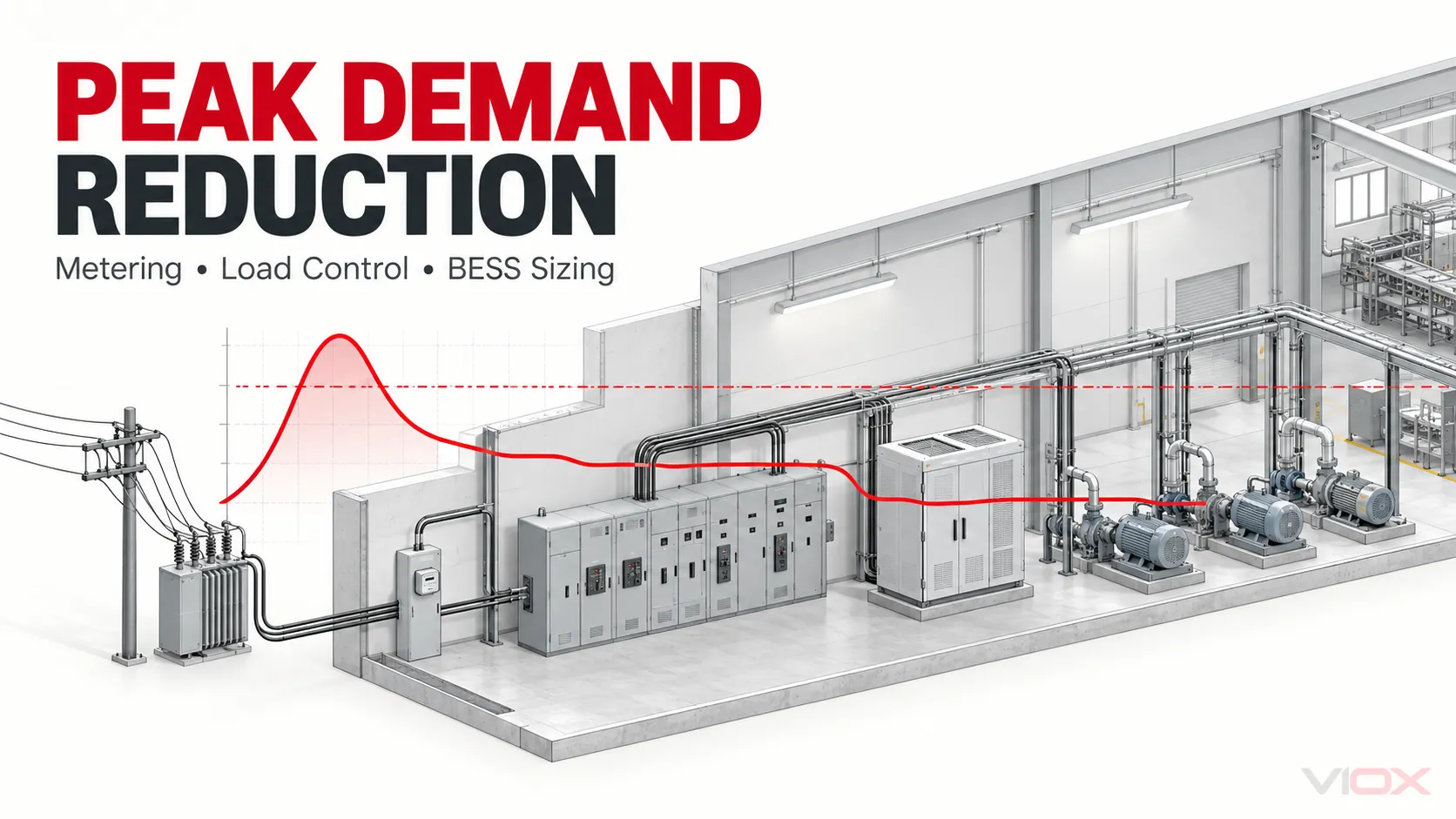
Pik talep azaltımı, bir ekipman seçimi probleminden önce bir aralık kontrolü problemidir. Elektrik tarifesi ve sayaç verileriyle başlayın, talep ücretini oluşturan miktarı yeniden yapılandırın, en yüksek ücretlendirilebilir aralıklardan sorumlu süreçleri tanımlayın ve ardından zamanlama, yük kontrolü ve enerji depolamanın en az kesintiye yol açan kombinasyonunu seçin.

Bir batarya enerji depolama sistemi (BESS), yalnızca güç dönüştürme sistemi anlık azaltmayı karşılayabildiğinde ve kullanılabilir enerjisi bu azaltmayı her ilgili olay için sürdürebildiğinde faydalıdır. Bu, varsayılan cevap değildir. Bir tesis; kademeli başlatmalar, yönetilen şarj, değişken frekanslı sürücü (VFD) ayar noktası kontrolü, termal yük zamanlaması, geçici yük atma, depolama veya koordineli bir kombinasyon yoluyla gerekli talep sınırını elde edebilir.

Mühendislik kapsamı: Aşağıdaki denklemler fizibilite analizini ve ön spesifikasyonu destekler. Faturayı elektrik tarifesi ve sayaç belirler. Detaylı tasarım; yine de geçerli elektrik yönetmeliğini, şebeke bağlantı kurallarını, koruma çalışmasını, yangın yönetmeliğini, ekipman dokümantasyonunu ve yetkili merciin (AHJ) onayını gerektirir.

1. Kontrol Edilmesi Gereken Miktarı Tanımlayın

Enerji ve talep birbiriyle ilişkilidir ancak birbirinin yerine kullanılamaz:

• Enerji, kWh: zaman içindeki güç entegrali.
• Talep, kW: tarifenin ölçüm yöntemi ve zaman aralığı altında belirlenen bir güç değeri.
• Görünür talep, kVA: bazı tarifelerde kW talebinin yerine veya buna ek olarak kullanılır.
• Faturalama talebi: zaman dilimleri, kademeli tarife, sözleşme gücü, güç faktörü düzeltmeleri veya eş zamanlı pik kuralları uygulandıktan sonra tarifenin fiilen kullandığı değer.

Basit bir sabit (T) süreli aralık için, (k) aralığındaki ortalama şebeke çekiş gücü şöyledir:

P_d,k = (1 / T) × ∫ P_grid(t) dt

Aralık enerji ithalatı (E_k) içeriyorsa, eşdeğer form şöyledir:

P_d,k = E_k / T

Maksimum aralığı yalnızca uygun bir zaman penceresi (W) içinde faturalandıran bir tarife için:

D_month = max(P_d,k), W içindeki her k aralığı için

Bu evrensel bir tarife tanımı değil, bir modeldir. Elektrik dağıtım şirketleri blok aralıklar, kayan aralıklar, termal talep, eş zamanlı sistem pikleri, çeşitli zaman dilimli talep kayıtları veya minimum/kademeli faturalama talebi kullanabilir. ABD Enerji Bakanlığı (DOE), kendi bünyesinde eş zamanlı olmayan talep, zaman dilimli talep, sistem pik talebi ve talep kademelerini birbirinden ayırır. şebeke tarifesi kılavuzu.

Ekipman analizinden önce çıkarılması gereken tarife girdileri

Tarife girdisi	Mühendislik sorusu	Kontrol tasarımını neden değiştirir
Talep miktarı	Talep kW, kVA veya her ikisi üzerinden mi faturalandırılıyor?	Bir kVA ücreti, sadece aktif güç azaltımını değil, güç faktörü analizini de gerektirebilir.
Aralık yöntemi	Blok, kayan, termal veya başka bir yöntem mi?	Kontrolör, faturalama değeri belirlenmeden önce harekete geçecek kadar yakın bir tahminle aynı miktarı hesaplamalıdır.
Ücretlendirilebilir pencere	Tüm saatler, yoğun saatler veya birkaç dönem mi?	Ücretlendirilebilir pencerenin dışındaki bir kontrol eyleminin talep ücreti değeri olmayabilir.
Cırcır/geriye dönük inceleme	Önceki talep bir faturalama tabanı oluşturuyor mu?	Daha düşük fiziksel zirveler faturayı hemen düşürmeyebilir.
Eş zamanlı pik	Ücretlendirme, tesis maksimumuna mı yoksa şebeke sistemi olaylarına mı dayanıyor?	Harici bir olayı tahmin etmek, tesis maksimumunu sınırlamaktan daha önemli olabilir.
İhracat kuralı	Ters güç akışına izin veriliyor mu ve nasıl ölçülüyor?	BESS kontrolcüsü bir ihracat kısıtlamasına ve ayrı bir ithalat/ihracat mantığına ihtiyaç duyar.
Sözleşme/minimum talep	Bir talep alt sınırı veya sözleşmeli kapasite var mı?	Bu taban değerin altına inmek, başka bir tarife avantajı sağlamayabilir.

Bu değerlerin hiçbirini tipik bir 15 dakikalık örnekten yola çıkarak tahmin etmeyin. Güncel tarife çizelgesini, ek maddeleri, özel koşulları ve son faturaları okuyun. Mümkünse, yorumunuzu elektrik dağıtım şirketi ile teyit edin.

2. Temel Çizgiyi Aralık Verilerinden Yeniden Oluşturun

Mevsimsellik, üretim karması, hava durumu veya tarife dönemlerinin puant değerini değiştirebileceği durumlarda en az bir tam işletme yılı verisi kullanın. Tarifenin daha uzun bir geriye dönük inceleme süresi varsa veya tesisin seyrek kampanyaları bulunuyorsa daha fazla veri gerekebilir.

Veri kalitesi kontrolleri

Puant değerlerini sıralamadan önce şunları doğrulayın:

1. Zaman damgası kuralı: yerel saat, UTC, yaz saati uygulaması geçişleri ve aralık sonu ile aralık başı zaman damgaları.
2. Aralık süresi: 5, 15, 30 ve 60 dakikalık kayıtları enerjiye göre yeniden örnekleme yapmadan karıştırmayın.
3. Eksik ve mükerrer kayıtlar: bunları işaretleyin; bir tepe aralığını sessizce ortalama bir değerle doldurmayın.
4. Birimler ve ölçeklendirme: Wh/kWh, W/kW, akım trafosu (CT) oranı, gerilim trafosu oranı ve çarpanı doğrulayın.
5. İthalat ve ihracat işareti: mümkün olduğunda bunları ayrı ayrı saklayın. Net bir değer, eş zamanlı yük ve üretim davranışını gizleyebilir.
6. Sayaç sınırı: ölçüm noktasının hangi besleyicilerin, jeneratörlerin ve depolama sistemlerinin yukarı veya aşağı yönünde olduğunu belirleyin.
7. Gelir mutabakatı: yeniden oluşturulan aylık pik değerleri ve toplam enerji miktarlarını faturalarla karşılaştırın. Kontrolleri boyutlandırmadan önce aradaki farkı açıklayın.

Dahili bir sayaç, gerçek zamanlı kontrol için paha biçilmezdir ancak gelir sayacının yerini tutmaz. Saati, toplama kuralı, CT hassasiyeti, örnekleme hızı ve sayaç sınırı sistematik bir fark yaratabilir. Ölçüm mimarisi ve doğruluk kavramları için VIOX kılavuzuna bakın: enerji sayaçları, CT'ler ve Modbus.

Sadece bir yük süresi eğrisi değil, bir pik olay tablosu oluşturun

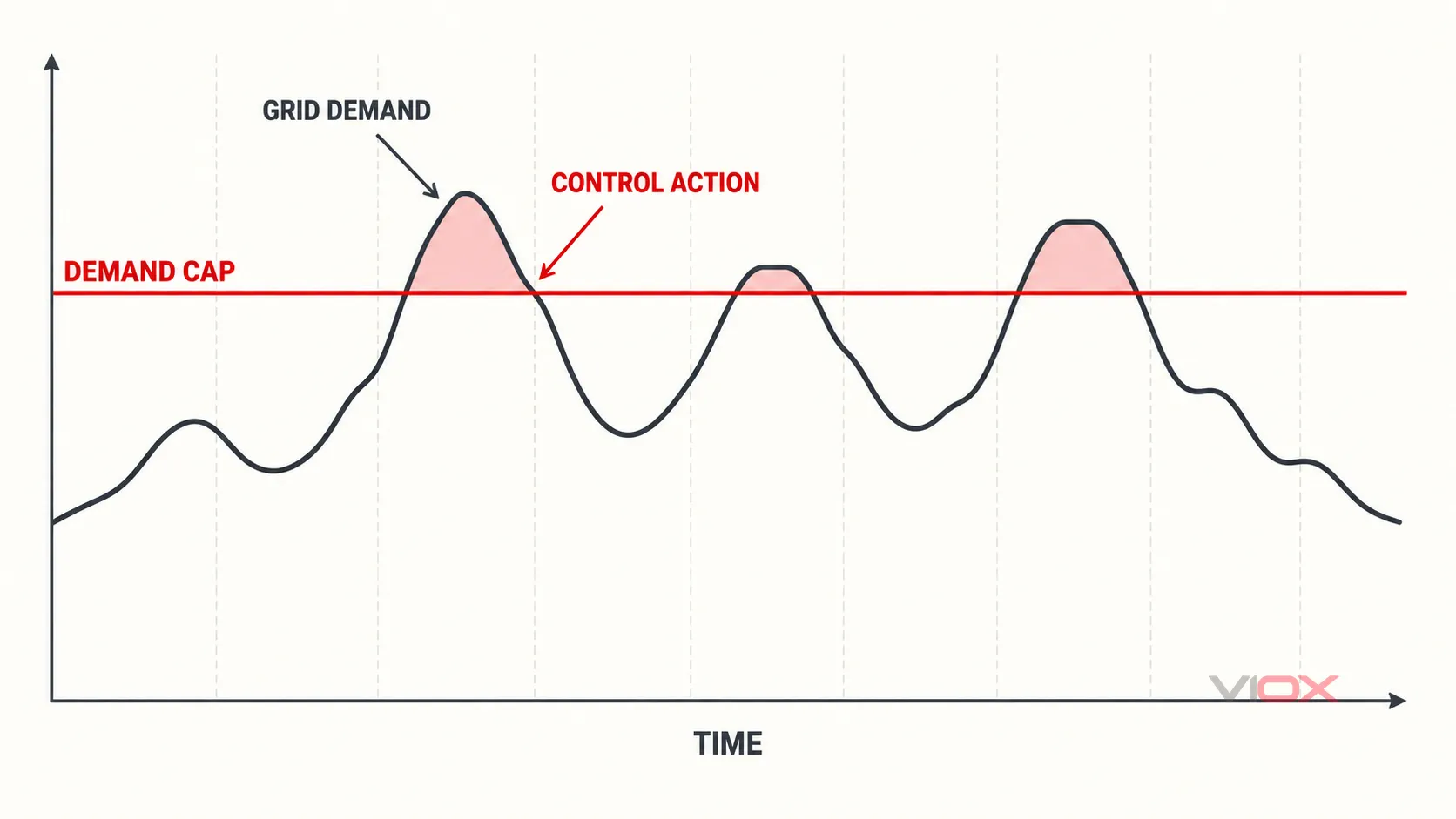
Bir yük süresi eğrisi, talebin bir eşiği ne sıklıkla aştığını gösterir ancak zaman sıralamasını kaldırır. Depolama boyutlandırma ve süreç kontrolü kronoloji gerektirir. Şunları içeren bir olay tablosu oluşturun:

• başlangıç ve bitiş zamanı;
• maksimum ve ortalama talep;
• aday sınırların üzerindeki süre;
• üretim durumu, parti, vardiya ve hava durumu bağlamı;
• büyük yük kalkışları ve çakışan görev döngüleri;
• kontrol edilebilir yük kullanılabilirliği;
• yerinde üretim ve depolama durumu;
• öncesindeki ve sonrasındaki toparlanma süresi.

Birbirine yakın aşılmaları tek bir olayda gruplandırın. Beş dakika ile ayrılan iki tepe noktası, batarya aralarında şarj olamıyorsa tek bir depolama görev döngüsü olabilir.

3. Beş Farklı Talep Stratejisini Ayırın

Her önlemi “tepe tıraşlama” olarak ele almak, önemli farkları gizler.

Strateji	Neler değişiyor	Enerji sonucu	Kontrol etkisi
Verimlilik	Aynı faydalı çıktı için gereken gücü azaltır	Genellikle kWh değerini düşürür ve tepe kW değerini azaltabilir	Kalıcı önlem; tasarrufun ücretlendirilebilir tepe aralıklarında gerçekleştiğini doğrulayın.
Yük kaydırma	Enerji tüketen bir görevi başka bir zamana erteler	Genellikle benzer toplam kWh	Program esnekliği ve güvenli bir yoğun olmayan saat aralığı gerektirir.
Yük atma	Bir yükü geçici olarak durdurur veya kısıtlar	Çıktıyı azaltabilir veya daha sonra telafi gerektirebilir	Öncelik, maksimum kesinti süresi ve yeniden başlatma mantığı gerektirir.
Pik tıraşlama	Şebeke alımını bir sınırın altında tutar	Enerjiyi kaydırabilir veya dönüşüm kayıpları ekleyebilir	Kapalı döngü ölçümü ve kontrol edilebilir yük, depolama veya üretim gibi bir aktüatör gerektirir.
Talep tarafı yönetimi	Bir şebeke veya piyasa olayına yanıt olarak yükü değiştirir	Sözleşmeye özel	Olay iletişimleri, temel kurallar, performans doğrulama ve operasyonel taahhüt gerektirir.

Oak Ridge Ulusal Laboratuvarı geçici olanı ayırt eder yük atma tüketimi şuradan kaydırarak yük kaydırma kendi elektrik faturası kılavuzu. DOE'nin endüstriyel talep yanıtı rehberi benzer şekilde, üretim yüklerini bir etkinlik yanıtına dahil etmeden önce tesisin yük profilini anlamanın önemini vurgular.

Önce düşük karmaşıklıktaki kontrolleri sıralayın

Teknik açıdan rasyonel bir sıra şöyledir:

1. ölçüm ve tarife modeli hatalarını ortadan kaldırın;
2. önlenebilir eş zamanlı kalkışları ve toparlanma piklerini giderin;
3. ertelenebilir yükleri yeniden planlayın;
4. esnek yükleri proses sınırları dahilinde modüle edin;
5. olağanüstü durumlarda onaylanmış yükleri devreden çıkarın;
6. operasyonel olarak yönetilemeyen bakiye için BESS veya başka bir sevk edilebilir kaynak kullanın.

Bu zorunlu bir ekonomik sıralama değildir. Bir depolama sisteminin, planlama düzeltmesi ile giderilebilecek pikleri karşılayacak şekilde boyutlandırılmasını önler.

4. Talep Sınırını Yüzdesel Bir Hedefe Göre Değil, Operasyonlara Göre Belirleyin

(m) ayı için yeniden oluşturulmuş faturalama talebi (D_{base,m}) olsun. Bir aday sınır değeri (P_{cap}), yalnızca kontrol sistemi proses, ekipman, tarife veya ara bağlantı kısıtlamalarını ihlal etmeden ilgili her bir aşımı karşılayabiliyorsa uygulanabilir.

Kontrolsüz net ithalat profilini şu şekilde tanımlayın:

P_base(t) = P_load(t) - P_onsite_generation(t)

İhracat yapmayan bir tesis için gerekli kontrol eylemi şudur:

P_control(t) = max(0, P_base(t) - P_cap)

Uygulanabilir kapasite simülasyon yoluyla bulunur. Kronolojik veriler üzerinde çeşitli kapasite değerlerini tarayın ve şunları kaydedin:

• kontrol olayı sayısı;
• maksimum kontrol gücü;
• olay başına gereken enerji;
• maksimum olay süresi;
• ardışık olaylar ve yeniden şarj fırsatı;
• kısıtlanmış üretim veya konfor etkisi;
• batarya verimi ve beklenen çalışma aralığı;
• tam tarife modeline göre kalan faturalandırma talebi.

Daha düşük bir üst sınır otomatik olarak daha iyi değildir. Bu durum olay sıklığını, depolama döngüsünü, süreç kesintisini ve bir tahmin veya iletişim hatasından sonra üst sınırı kaçırma riskini artırabilir.

5. Tahminleyici Aralık Kontrolü Kullanın

Yalnızca ölçülen talep hedefi aştıktan sonra tepki veren bir kontrolör çok geç kalabilir. (T) süreli bir aralıkta, (t) geçen süresinde, (E_{elapsed}) mevcut aralıkta biriken ithal enerji ve (P_{now}) kalan aralık için tahmin edilen net ithalat olsun. Basit bir projeksiyon şöyledir:

P_projected = [E_elapsed + P_now × (T - t)] / T

Sınır altındaki kalan enerji payı şudur:

E_headroom = P_cap × T - E_elapsed

Tutarlı birimler kullanın: güç kW ve enerji kWh cinsinden ise, (T) ve (t) değerlerini saat cinsinden ifade edin.

Öngörülen talep sınırı aşarsa, kontrolör mevcut kaynakları önceliğe göre dağıtır. Uygulamada, sağlam bir tahminleyici şunları dikkate almalıdır:

• gelir sayacı aralık senkronizasyonu;
• sayaç ve haberleşme gecikmesi;
• yük artış hızı ve tahmin hatası;
• aktüatör tepki süresi;
• VFD minimum hız ve proses kısıtlamaları;
• kontaktör anahtarlama görevi ve minimum açma/kapama süresi;
• kompresör, soğutma grubu, fırın veya pompa yeniden başlatma kısıtlamaları;
• BESS şarj durumu (SOC), sıcaklık, güç limitleri ve yedek;
• titremeyi önlemek için histerezis veya ölü bant;
• sensör, ağ veya kontrolör arızasından sonra yedek davranış.

Bir anahtarlama kontaktörünü yüksek frekanslı modülasyon elemanı olarak kullanmayın. Motor tahrikli bir prosesin sürekli ayar noktası düzenlemesine uygun olduğu durumlarda bir VFD kullanın ve anahtarlama frekansını ekipmanın doğrulanmış görev döngüsü içinde tutun. VIOX açıklayıcıları şunlardır: VFD çalışma prensipleri ve kontaktör anahtarlama fonksiyonu bileşen düzeyinde arka planı sağlayın.

6. Yük Öncelik Matrisi Oluşturun

Her kontrol edilebilir yükün belgelenmiş bir operasyonel sözleşmeye ihtiyacı vardır. “Kapatılabilir” ifadesi yeterli değildir.

Alan	Gerekli tanım
Yük kimliği ve ölçüm noktası	Hangi besleyicinin veya sürecin kontrol edildiği ve yanıtının nasıl doğrulandığı
Kontrol modu	Başlatma engelleme, program kaydırma, kademeli kapatma, ayar noktası düşürme veya güç sınırı
Mevcut azaltım	Sadece etiket değerine göre değil, çalışma durumunun bir fonksiyonu olarak beklenen kW
Yanıt süresi	Komuttan ölçülebilir şebeke azaltımına kadar geçen gecikme
Minimum/maksimum durum	Güvenli minimum hız, sıcaklık, basınç, debi, SOC veya çıkış
Maksimum kesinti	Ürün, güvenlik, konfor veya ekipman limitleri etkilenmeden önceki süre
Yeniden başlatma davranışı	Ani akım, ısınma, sıralama, geri tepme talebi ve minimum kapalı kalma süresi
Öncelik	Asla kısıtlamayın, önce modüle edin, erteleyin veya yalnızca son çare olarak kesin
Arıza emniyetli durum	Sayaç verisi, haberleşme, kontrolör veya aktüatör gücü kaybından sonraki sonuç

Güvenlik sistemleri, koruma fonksiyonları, acil durum havalandırması, can güvenliği yükleri ve kesintiye uğraması tehlikeli bir proses durumuna yol açan yükler, yetkili bir tasarım makamı tarafından açıkça entegre edilmedikçe olağan talep azaltma mantığının dışındadır.

7. Talep Kontrol Sistemi Mimarisi

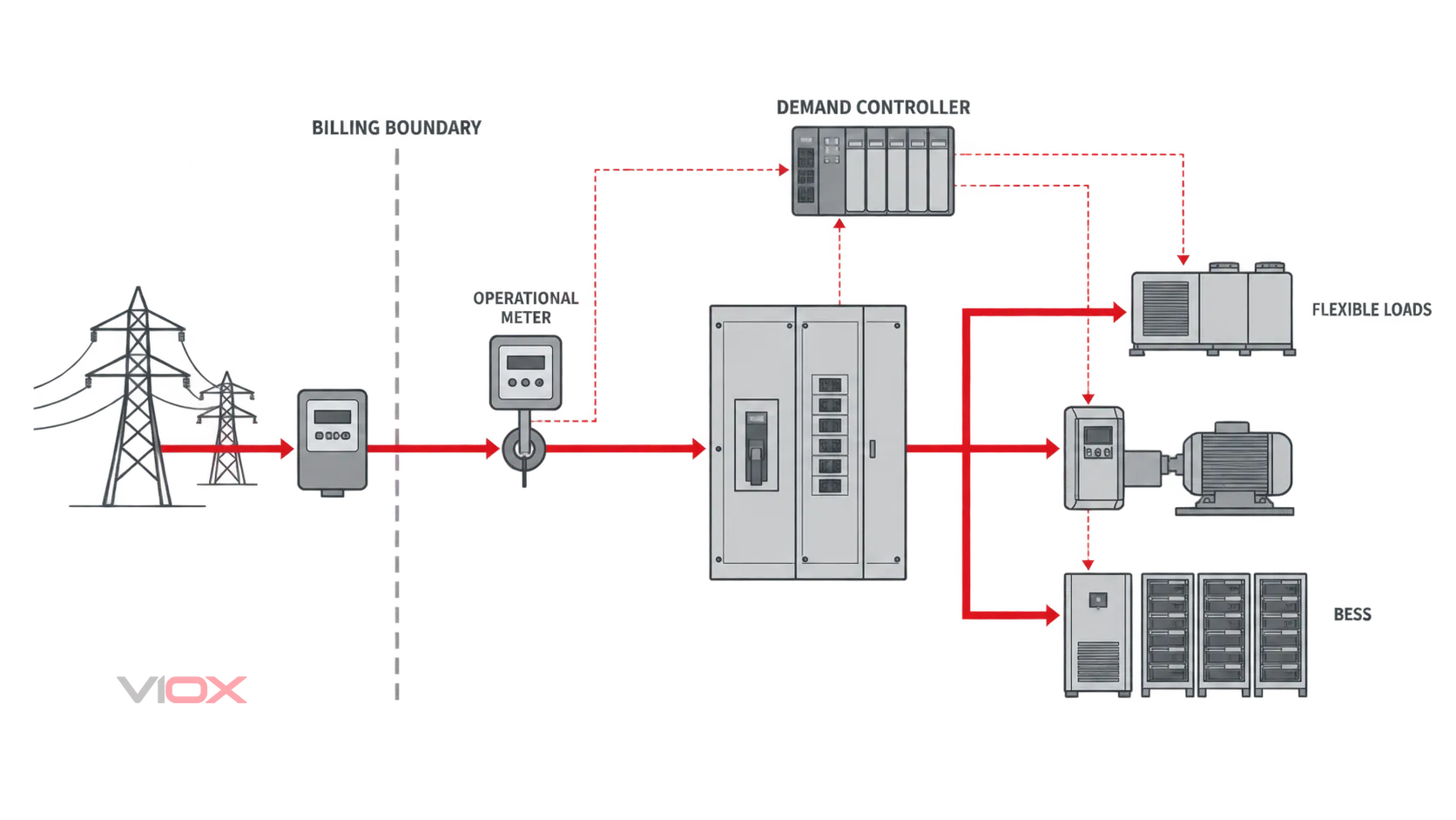
Tipik bir mimari beş fonksiyonel katmana sahiptir:

1. Faturalandırma sınırı: şebeke gelir sayacı ve aktif tarife ücreti belirler.
2. İşletimsel ölçüm: bir tesis sayacı, doğru ölçeklendirilmiş akım trafoları (CT), alt ölçümleme ve zaman senkronizasyonu; kontrol ve teşhis için daha hızlı veri sağlar.
3. Talep tahmincisi: bir enerji yönetim sistemi (EMS), programlanabilir mantıksal denetleyici (PLC) veya özel bir kontrolör, aralık talebini yeniden oluşturur ve aralık sonunu tahmin eder.
4. Dağıtım mantığı: öncelik, süreç izinleri, SOC sınırları, ölü bant, dışa aktarım kısıtlaması ve arıza emniyet kuralları eylemi belirler.
5. Aktüatörler: zamanlama sistemleri, VFD ayar noktaları, yönetilen elektrikli araç şarjı, kumanda röleleri/kontaktörler, izin verilen yerlerde jeneratör kontrolleri ve BESS güç dönüşüm sistemi (PCS).

Güç koruması, optimizasyon hedefinden bağımsız kalır. Talep kontrolcüsü; aşırı akım korumasının, toprak hatası korumasının, ada oluşumunu önleme fonksiyonlarının, acil durdurmanın veya ekipmana özel güvenlik kontrollerinin yerini almaz.

8. BESS Güç ve Enerji Boyutlandırmasını Ayrı Ayrı Yapın

Batarya gücü ve batarya enerjisi farklı kısıtları çözer. Makale kW, kWh, MW, MWh, SOC ve deşarj derinliği bu terimleri ayrıntılı olarak açıklar.

8.1 PCS güç değeri

Zaman serisi fizibilite modeli için gerekli AC deşarj gücü şöyledir:

P_BESS,AC(t) = max(0, P_base(t) - P_cap - P_flexible_load(t))

Burada (P_{flexible_load}(t)), temel çizgiye göre planlama, modülasyon veya onaylı yük atma yoluyla sağlanan pozitif bir azalma olarak tanımlanır.

Ön PCS deşarj değeri, gereken maksimum değerden en az şu kadar olmalıdır:

P_PCS,discharge ≥ max[P_BESS,AC(t)]

Nihai PCS spesifikasyonu ayrıca aşırı yük kapasitesi ve süresini, sıcaklık ve rakım değer kaybını, reaktif güç görevini, ithalat/ihracat kısıtlamalarını, transformatör ve iletken kapasitesini, arıza katkısını, harmonik performansını ve ara bağlantı sözleşmesini dikkate almalıdır. PCS'nin tanımlanmış bir pencere içinde yeniden şarj olması gerekiyorsa, şarj gücü ayrı bir gerekliliktir.

8.2 Bir olay sırasında iletilen enerji

(j) olayı için, gereken AC enerjisi, esnek yük kontrolünden sonra üst sınırın üzerindeki alandır:

E_AC,event,j = ∫ P_BESS,AC(t) dt

En kötü olası olayı ön bir etiket enerjisine dönüştürün:

E_nameplate ≥ E_AC,event / (η_dis × f_usable × f_EOL)

nerede:

• (η_{dis}), ilgili çalışma aralığı boyunca modellenen deşarj yolu verimliliğidir;
• (f_{usable}), çalışma SOC sınırları arasındaki etiket enerjisinin izin verilen kısmıdır;
• (f_{EOL}), tasarım ömrü sonunda gerekli olan korunan kapasite oranıdır.

Önemli olduğunda zaman serisi modeline yardımcı yükleri ve sıcaklık etkilerini dahil edin. Gizli muhafazakar varsayımların üzerine açıklanmamış bir “emniyet faktörü” eklemeyin; her bir payı bir kez belirtin.

8.3 Kronoloji, enerji değerini belirleyebilir

15 dakikalık bir talep aralığı, 0,25 saatlik bir bataryanın yeterli olduğu anlamına gelmez. Bir tesis, art arda birkaç aralık boyunca sınırın üzerinde kalabilir. Ayrıca batarya toparlanmadan önce ikinci bir olay yaşayabilir. Şunları simüle edin:

• sürekli çoklu aralık tepe değerleri;
• şarj gücü ve izin verilen şarj süreleri;
• yeni bir talep zirvesi yaratan şarj;
• minimum SOC rezervi;
• tahmin hatası;
• analiz dönemi boyunca bozulma;
• uygulanabilirse eş zamanlı reaktif güç gereksinimleri.

NREL’in System Advisor Model batarya dokümantasyonu tepe tıraşlama kontrolcüleri dahil olmak üzere zaman serisi dağıtımını destekler ve sıcaklık ile bozulma etkilerini modeller. Bir yatırım kararı için uygun analiz seviyesi budur; tek bir aylık maksimum değer yeterli değildir.

9. Uygulamalı Örnek: PCS kW ve Ön Batarya kWh Değerlerini Türetme

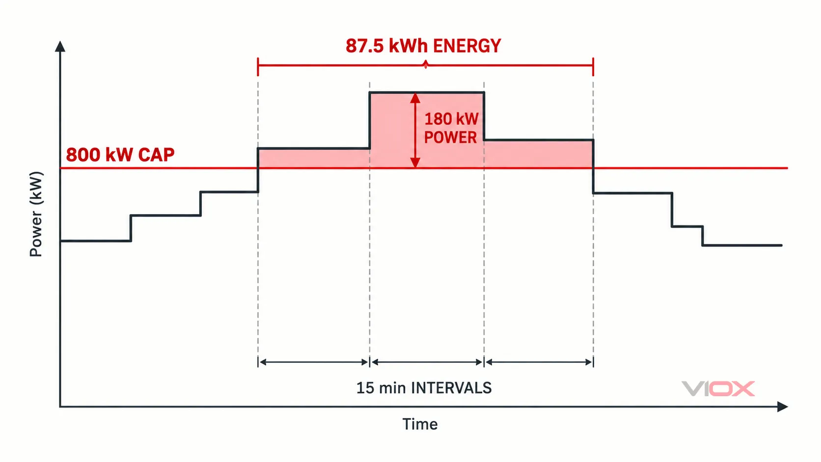
15 dakikalık basit bir blok talep tarifesi, kademesiz (no ratchet), ihracatsız ve 800 kW'lık bir aday talep sınırı varsayın. Onaylanan tüm esnek yük eylemlerinden sonra, birbirini izleyen beş aralık ortalaması net ithalat şöyledir:

Ara	Baz ithalat (kW)	Gerekli BESS deşarjı (kW)
1	720	0
2	860	60
3	980	180
4	910	110
5	760	0

Her aralığın tam 0,25 saat boyunca listelenen ortalamada kaldığını varsayın. Bu olaydan kaynaklanan minimum güç gereksinimi şudur:

P_PCS,discharge ≥ max(60, 180, 110) = 180 kW

Sağlanan AC enerjisi şöyledir:

E_AC,event = (60 + 180 + 110) kW × 0.25 h
           = 87.5 kWh

0,94'lük açıklayıcı bir deşarj verimliliği, 0,80'lik kullanılabilir SOC oranı ve 0,80'lik kullanım ömrü sonu kapasite koruma oranı için:

E_nameplate ≥ 87.5 / (0.94 × 0.80 × 0.80)
            ≥ 145.4 kWh

Bu nedenle ön sonuç, en az 180 kW PCS deşarj kapasitesi ve 145.4 kWh etiket enerjisidir bu basitleştirilmiş olay ve bu varsayımlar için. Bu bir tedarik şartnamesi değildir. Kronolojik bir yıllık simülasyon; daha uzun bir olay, yetersiz şarj aralığı, daha yüksek güç rampası, daha düşük verimlilik veya gerçek değeri belirleyen işletme rezervi ortaya çıkarabilir.

10. Tasarruf Sözü Vermeden Tarife Sonucunu Modelleme

Tek bir basit aylık talep tarifesi (R_m) için başlangıç talep ücreti modeli şöyledir:

Yıllık talep ücreti indirimi = Σ [R_m × (D_base,m - D_controlled,m)]

Tarife; kademeli artışlar, birden fazla talep dönemi, çakışan pikler, kVA talebi, sözleşme taban fiyatı, yedekleme ücretleri veya kademeli talep oranları içerdiğinde bu ifadeyi olduğu gibi kullanmayın. Faturayı kalem kalem yeniden oluşturun.

Teknik-ekonomik model şunları içermelidir:

• her tarife kaydı altında kontrollü talep;
• farklı fiyat dönemlerine kaydırılan enerji;
• BESS gidiş-dönüş kayıpları ve yardımcı tüketim;
• batarya bozulması ve değişim varsayımları;
• bakım ve haberleşme maliyetleri;
• yük kısıntısından kaynaklanan üretim etkisi;
• yalnızca imzalı bir programın temel çizgiyi ve performans kurallarını tanımladığı durumlarda talep tarafı katılım geliri;
• tahmin veya ekipman arızası sonrası artık talep riski.

Tarifeye duyarlılık, pik şekli, üretim programı, batarya ömrü ve kapasite uyumluluğu hakkında rapor verin. Evrensel bir tasarruf yüzdesi veya geri ödeme süresi teknik olarak savunulabilir değildir.

11. Elektrik, Şebeke Bağlantısı ve Güvenlik Sınırları

Talep azaltımı, tam bir elektrik sistemi tasarımı ihtiyacını ortadan kaldırmaz. En azından şunları doğrulayın:

• hem şarj hem de deşarj durumlarında servis ve transformatör yüklemesi;
• kısa devre akımı, koruma koordinasyonu, topraklama, izolasyon ve acil durdurma;
• akım trafosu (CT) polaritesi, oranı, sınıfı, yükü, sayaç hassasiyeti ve sinyal kaybı davranışı;
• PCS gerilimi, frekansı, harmonikler, reaktif güç modu, arıza tepkisi ve ada modu koruması (anti-islanding) gereksinimleri;
• ihracat sınırlaması ve şebeke bağlantı onayı;
• pano konumu, havalandırma veya termal yönetim, erişim, açıklıklar ve çevresel koşullar;
• batarya yönetim sistemi limitleri, alarmlar, yangın algılama, devreye alma ve acil durum müdahalesi;
• ağa bağlı sayaçlar, EMS, PLC, EVSE ve PCS arayüzleri için siber güvenlik ve erişim kontrolü.

ABD projeleri için ilgili kapsam referansları şunları içerebilir: sabit enerji depolama kurulumu için NFPA 855, enerji depolama sistemleri ve ekipmanları için UL 9540ve DER ara bağlantısı ve birlikte çalışabilirlik için IEEE 1547. Kabul edilen sürümler ve uygulanabilirlik; yargı yetkisine, sistem konfigürasyonuna ve AHJ'ye bağlıdır. Diğer ülkeler farklı yasal düzenlemeler ve standartlar çerçeveleri kullanmaktadır.

12. Devreye Alma ve Ölçüm-Doğrulama Planı

Devreye alma işlemi, sadece münferit cihazların haberleştiğini değil, tüm kontrol zincirinin çalıştığını kanıtlamalıdır.

Sayaç ve model kabulü

• Akım trafosu (CT) yönünü, ölçeklendirmeyi, zaman senkronizasyonunu ve import/export işaretini doğrulayın.
• İşletme sayacı aralık enerjisini ve talebini, temsili dönemler boyunca şebeke verileriyle karşılaştırın.
• Kontrol cihazının aralıkları hedeflenen tarife modeline göre sıfırladığını ve topladığını onaylayın.
• Eksik verileri, dondurulmuş değerleri, aralık dışı okumaları ve saat arızasını test edin.

Kontrol kabulü

• Uygulanabilir olduğu durumlarda, gerçek talep sınırının altında kontrollü bir test profili uygulayın.
• Öngörülen talebi, devreye alma eşiğini, ölü bandı ve bırakma eşiğini onaylayın.
• Her esnek yük için gerçek kW düşüşünü ve tepki süresini ölçün.
• Minimum açma/kapama süresini, yeniden başlatma sırasını, geri tepme talebini ve süreç izinlerini doğrulayın.
• İletişim veya kontrolör gücü kaybının, belgelenmiş güvenli durum (fail-safe) ile sonuçlandığını onaylayın.

BESS kabulü

• Komut verilen AC gücü ve enerjisi ile ölçülen değerleri doğrulayın.
• SOC sınırlarını, rezervi, dışa aktarım kısıtlamasını, şarj geri kazanımını, alarmları ve acil durdurmayı test edin.
• Şarj zamanlamasının yeni bir ücretlendirilebilir tepe noktası oluşturmadığını onaylayın.
• Modellenen en uzun olayı veya onaylanmış eşdeğer bir testi gösterin.

Fatura doğrulama

• Kontrollü aralık verilerini kullanarak her aylık faturayı yeniden oluşturun.
• Fiziksel pik düşüşünü faturalandırılan talep düşüşü ile karşılaştırın; kademeli artış veya tarife taban etkilerini inceleyin.
• Kapasite aşımı hatalarını nedenlerine göre takip edin: tahmin, sayaç, iletişim, kullanılamayan yük, SOC, ekipman açması veya operatör müdahalesi.
• Malzeme üretimi, tarife, üretim veya ekipman değişikliklerinden sonra kronolojik modeli yeniden çalıştırın.

Bu sürecin sonucu sadece bir gösterge panelindeki daha küçük bir pik değildir. Bu; tarife tanımından ölçülen aralığa, kontrol kararına, fiziksel yük yanıtına ve doğrulanmış faturalama sonucuna kadar izlenebilir bir zincirdir.

Kaynaklar

• DOE FEMP: Hizmet Tarifesi Seçeneklerinizi Değerlendirme
• DOE Better Plants: Endüstriyel Tesislerde Talep Tarafı Yönetimi
• ORNL: Elektrik Faturalarınızı Anlamak—Elektrik
• NREL Sistem Danışman Modeli: Batarya Depolama
• NFPA 855: Sabit Enerji Depolama Sistemlerinin Kurulumu Standardı
• UL 9540: Enerji Depolama Sistemi Testi ve Sertifikasyonu
• IEEE 1547-2018: Dağıtık Enerji Kaynaklarının Ara Bağlantısı ve Birlikte Çalışabilirliği